
CView: Crystal Structure Visualization & Analysis
![]()
![]()
CView is a high-performance crystallographic tool written in Rust and GTK4. It bridges the gap between structure visualization and ab-initio calculation setup (VASP, QE, SPRKKR).
This version of CView is built on GTK4, which primarily utilizes the CPU for rendering.
While the engine is optimized, it is designed for crystal structures (unit cells, supercells, slabs). It handles systems up to $\approx 1000$ atoms with ease, but it is not suitable for visualizing massive biological macromolecules (e.g., proteins, DNA) containing millions of atoms.
CView is not just a viewer; it is a pre-calculation validator. It focuses on Reciprocal Space and Geometric consistency to prevent wasted CPU hours on incorrect VASP/QE inputs.
⚡ Why CView?
| Feature | Description |
|---|---|
| Fast & Lightweight | Built on Rust/GTK4. No GPU drivers required. Runs on any laptop. |
| Analysis First | Dedicated tools for K-Paths, Slabs, and Void Analysis. |
| DFT Ready | Native support for VASP, Quantum Espresso, and SPRKKR formats. |
| Publication Quality | Export high-resolution, transparent PNGs and PDFs using PBR rendering. |
Documentation Overview
This manual is divided into three parts:
- Installation: Get CView running on Linux, Windows, or macOS.
- User Guide: Deep dive into the scientific methodology.
- K-Path Visualization: Brillouin zone construction and HSP selection.
- XRD Simulation: Structure factors and powder diffraction patterns.
- Surface Slabs: Creating vacuum-padded slabs for surface science.
- Tutorials: Step-by-step walkthroughs for real materials (e.g., Bi₂Se₃).
Quick Start
Get up and running in seconds.
# Clone and Run
git clone https://github.com/mavensgroup/cview.git
cd cview
cargo run --release
See the Installation Page for detailed OS-specific instructions.
Supported Formats
| Format | VASP | Quantum Espresso | SPRKKR | CIF / XYZ |
|---|---|---|---|---|
| Read | 🟢 | 🟢 | 🟢 | 🟢 |
| Write | 🟢 | 🟠 | 🟠 | 🟢 |
| Relaxation | 🟢 | 🟢 | 🔴 | 🔴 |
Links
This is an α (alpha) release. While the core functionality is operational, the software may contain incomplete features, bugs, or unstable behaviour.
Contributions from testers and developers are welcome.
📜 License & Citation
CView is open-source software licensed under the LGPLv3.
If you use CView in your research, please cite the repository.
Installation
If you have cargo installed, then jump to Build from source.
CView is a cross-platform application built on Rust and GTK4. Because it uses the native GTK4 libraries for rendering, the installation process involves two steps:
- Installing the system dependencies (GTK4).
- Compiling the application using Cargo.
1. Install Dependencies
Select your operating system below to set up the required libraries.
Linux
You need the GTK4 development headers and the standard build tools (gcc/clang).
Fedora / RHEL
sudo dnf install gcc gtk4-devel libadwaita-devel
Ubuntu / Debian / Mint
sudo apt update
sudo apt install build-essential libgtk-4-dev libadwaita-1-dev
Arch Linux / Manjaro
sudo pacman -S base-devel gtk4 libadwaita
macOS
The easiest way to install GTK4 on macOS is via Homebrew.
# 1. Install Homebrew if you haven't already
/bin/bash -c "$(curl -fsSL [https://raw.githubusercontent.com/Homebrew/install/HEAD/install.sh](https://raw.githubusercontent.com/Homebrew/install/HEAD/install.sh))"

# 2. Install Rust and GTK4
brew install rust gtk4 libadwaita adwaita-icon-theme
Windows
For Windows, we recommend using the MSYS2 environment to manage the native GTK4 libraries.
- Install MSYS2: Download the installer from msys2.org.
- Open the Terminal: Launch
MSYS2 MinGW 64-bit. - Install Toolchain:
Run this command inside the MSYS2 terminal:
pacman -S mingw-w64-x86_64-gtk4 mingw-w64-x86_64-rust mingw-w64-x86_64-gcc - Add to Path: Add
C:\msys64\mingw64\binto your Windows System PATH environment variable.- Why? This allows you to run
cargo runfrom VS Code or PowerShell later.
- Why? This allows you to run
The pacman command above works only inside the MSYS2 terminal. It will fail if you try to run it in PowerShell or Command Prompt.
2. Install Rust
If you do not have the Rust compiler installed, the recommended way is via rustup.
Command (Linux / macOS / Windows PowerShell):
curl --proto '=https' --tlsv1.2 -sSf [https://sh.rustup.rs](https://sh.rustup.rs) | sh
3. Build from Source
Once the dependencies are ready, you can compile CView directly from the repository.
# 1. Clone the repository
git clone [https://github.com/mavensgroup/cview.git](https://github.com/mavensgroup/cview.git)
cd cview

# 2. Build and Run (Release mode recommended for performance)
cargo run --release
This will install cview in ~/bin by default. For the subsequent run, just type cview
The first compilation may take a few minutes as it compiles the dependencies. Subsequent runs will be instant.
Troubleshooting
If the build fails claiming it cannot find gtk4 or pkg-config, it means the development headers are missing.
- Linux: Ensure you installed the
-devor-develpackages (e.g.,libgtk-4-dev), not just the runtime library. - macOS: Try running
brew link gtk4.
If you see errors related to cc or ld:
- Ensure you have
build-essential(Linux) or Xcode Command Line Tools (macOS) installed.
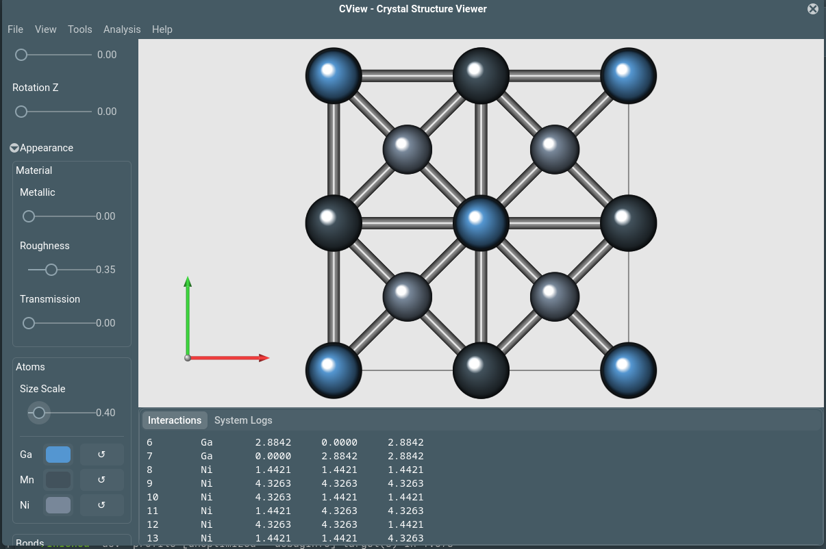
Loading & Visualization
This section outlines the core workflows for importing structure files, managing the workspace, and controlling the visual representation of crystal structures.
File Operations
Opening Files
To load a structure, navigate to File → Open (Ctrl + O) in the application menu. CView utilizes the native file chooser of your operating system to ensure a familiar experience.
Supported Formats: CView automatically detects the file type based on extension and content. You can open the following formats:
| Format | Extensions | Description |
|---|---|---|
| CIF | .cif | Standard Crystallographic Information Files. |
| VASP | POSCAR, CONTCAR, .vasp | Standard VASP structure inputs and outputs. |
| Quantum Espresso | .in, .out, .pwi, .qe | Reads atomic positions and cell parameters from input/output logs. |
| SPR-KKR | .pot, .sys | Munich SPR-KKR potential and system files. |
| XYZ | .xyz | Cartesian coordinates (Standard and Extended XYZ). |
Tab Management
CView uses a tabbed interface to handle multiple structures simultaneously. The application employs a smart loading strategy to keep the workspace clean:
- Replacement Mode: If the current active tab is empty (labelled "Untitled" with no structure), opening a file will replace this tab.
- New Tab Mode: If a structure is already loaded, the new file will open in a separate, closable tab.
Upon successfully loading a file, the application logs the event in the Interaction Log and automatically refreshes the Sidebar to display the atom list for the new structure.
Saving & Exporting
Saving Data
To convert a loaded structure into a different format, use File → Save As (Shift+ Ctrl+ S). The output format is determined by the selected file filter in the dialog.
Available Output Formats:
- CIF (*.cif)
- VASP POSCAR (POSCAR, *.vasp)
- SPR-KKR Potential (*.pot)
- Quantum Espresso Input (*.in)
- XYZ (*.xyz)
Visualization Controls
Once a structure is loaded, the View menu provides tools to orient and inspect the crystal lattice.
Standard Views
Quickly align the camera to specific crystallographic axes to inspect symmetry or stacking sequences.
- View Along A: Aligns camera with the a-axis (y=−90°).
- View Along B: Aligns camera with the b-axis (x=90°).
- View Along C: Aligns camera with the c-axis (Standard Plan View).
- Reset View: Restores the default zoom (1.0) and rotation (0,0).
Rotation Modes
You can customize the pivot point around which the camera rotates, depending on whether you are inspecting the atomic cluster or the lattice boundaries.
| Mode | Description |
|---|---|
| Centroid | Rotates around the geometric centre of the atoms. Best for inspecting molecules or specific bonding environments. |
| Unit Cell | Rotates around the centre of the unit cell box. Best for understanding the lattice boundaries relative to the origin. |
Exporting Visuals
For publications and presentations, CView offers high-fidelity export options via the File → Export (Ctrl + E) menu.
PNG Image: Renders a high-resolution raster image (default resolution: $2000\times 1500$ pixels). Ideal for slides and quick sharing.
PDF Document: Exports the scene as a vector graphic. This is recommended for academic papers, as it allows for infinite scaling without loss of quality.
Analysis Tools
The Analysis module in CView aggregates tools designed to characterize the geometric, symmetric, and diffraction properties of the loaded crystal structure. Unlike simple visualization, these tools perform computational tasks to extract physical descriptors suitable for comparison with experimental data or preparation for ab initio calculations.
Accessing Analysis Tools
The analysis suite is accessible via the Analysis menu in the main application window. This triggers the centralized Analysis Window (actions_analysis.rs), which provides tabbed access to the following modules:
- Symmetry: Space group determination and symmetry operation analysis.
- XRD: X-Ray Diffraction pattern simulation.
- Voids: Porosity and intercalation site analysis.
- K-Path: Reciprocal space path generation for band structures.
Documentation Modules
Detailed physical derivation and algorithmic implementation for each tool are provided below:
- Symmetry Analysis
- Engine: Moyo (Rust implementation of Spglib).
- Output: Space Group symbols, numbers, and crystal systems.
- XRD Simulation
- Theory: Kinematic Diffraction Theory.
- Features: Powder patterns, Cu-K$\alpha$ radiation, Lorentz-Polarization corrections.
- Void & Intercalation
- Method: Grid-based geometric insertion.
- Application: Porosity calculation and battery ion insertion sites.
- Reciprocal Space (K-Path)
- Method: High-symmetry path standardization (Setyawan-Curtarolo).
- Application: Band structure calculation inputs.
Note: While Surface Slabs are technically a structural building operation, their documentation regarding miller index transformation is provided here for completeness.
- Surface Slabs
- Method: Lattice transformation via planar basis searching.
Symmetry Analysis
The Symmetry module identifies the underlying crystallographic space group of the loaded structure. It is essential for reducing computational cost in DFT calculations and validating experimental structures.
Algorithmic Implementation
CView utilizes the Moyo library (a Rust ecosystem equivalent to Spglib) to perform symmetry determination. The analysis pipeline proceeds as follows:
- Lattice Standardization: The internal
Structure(Cartesian coordinates) is converted into aMoyo::Cell, utilizing the lattice vectors as columns of a $3\times3$ matrix. - Coordinate Transformation: Atomic positions are transformed from Cartesian ($r_{cart}$) to Fractional ($r_{frac}$) coordinates via the inverse lattice matrix: $$r_{frac} = M_{lattice}^{-1} \cdot r_{cart}$$
- Symmetry Search: The algorithm searches for symmetry operations (rotations $R$ and translations $t$) that map the crystal onto itself: $$R \cdot r + t \equiv r' \pmod 1$$ where $r$ and $r'$ are atomic positions of the same species.
Tolerance (SYMPREC)
The code applies a default symmetry precision (SYMPREC) of 1e-3 Å. This tolerance accommodates minor numerical noise common in file formats like .cif or .xyz, ensuring that slightly distorted experimental structures are correctly identified.
Outputs
The module returns a SymmetryInfo struct containing:
- Space Group Number: The International Tables for Crystallography (ITA) number (1–230).
- International Symbol: The Hermann-Mauguin notation (e.g., $Pm\overline{3}m$, $Fm\overline{3}m$).
- Crystal System: The classification (Triclinic, Monoclinic, Orthorhombic, Tetragonal, Trigonal, Hexagonal, or Cubic).
Usage Reference
This analysis is performed "read-only" regarding the structure; it calculates descriptors without altering the atomic coordinates of the active tab.
XRD Simulation
The X-Ray Diffraction (XRD) module simulates the powder diffraction pattern for the loaded structure. It utilizes Kinematic Diffraction Theory, assuming ideal interactions without primary extinction or multiple scattering events.
Physical Model
1. Lattice Physics
The simulation first calculates the Reciprocal Lattice vectors ($b_1, b_2, b_3$) from the real space lattice ($a_1, a_2, a_3$): $$b_1 = 2\pi \frac{a_2 \times a_3}{a_1 \cdot (a_2 \times a_3)}$$ (and cyclic permutations for $b_2, b_3$).
2. Bragg Condition
The code iterates through integer Miller indices $(h, k, l)$ to find reciprocal lattice vectors $G_{hkl} = h b_1 + k b_2 + l b_3$. The d-spacing is calculated as: $$d_{hkl} = \frac{2\pi}{|G_{hkl}|}$$ Diffraction peaks are identified where the Bragg condition is met for the source wavelength ($\lambda = 1.5406 Å$, Cu K$\alpha$): $$\lambda = 2d \sin\theta$$
3. Structure Factor ($F_{hkl}$)
The intensity of each reflection is governed by the Structure Factor, calculated by summing over all $N$ atoms in the unit cell: $$F_{hkl} = \sum_{j=1}^{N} f_j(\theta) \exp\left[2\pi i (hx_j + ky_j + lz_j)\right]$$
- $x_j, y_j, z_j$: Fractional coordinates of atom $j$.
- $f_j(\theta)$: The atomic scattering factor.
The atomic scattering factor ($f_j(\theta)$) has been calculated using Cromer-Mann coefficient (model/elements.rs)
4. Intensity Correction
The raw squared structure factor $|F_{hkl}|^2$ is corrected to obtain the observed intensity $I$. The primary correction applied in xrd.rs is the Lorentz-Polarization (LP) Factor for unpolarized radiation (standard laboratory diffractometer):
$$ \begin{align} LP(\theta) &= \frac{1 + \cos^2(2\theta)}{\sin^2\theta \cos\theta}\\ I_{calc} &= |F_{hkl}|^2 \times LP(\theta) \end{align}$$
5. Multiplicity and Merging
In powder diffraction, symmetry-equivalent planes (e.g., $(100)$ and $(010)$ in cubic systems) diffract at the same angle. The code algorithmically sorts peaks by $2\theta$ and merges peaks falling within a narrow tolerance ($0.05^\circ$), summing their intensities to account for multiplicity.
6. Match with Experiment
You can load the experimental ascii/xlsx file to compare the xrd using the "Load Experiment" button.
Settings
- Wavelength: Default fixed to Cu K$\alpha$ ($1.5406 Å$).
- Range: $10^\circ$ to $90^\circ$ $2\theta$.
- Filtering: Peaks with intensity $\leq 10^{-4}$ relative to the maximum are discarded to reduce noise.
High symmetry k-points and k-path
Electronic structure calculations (Band Structures) requires sampling the energy eigenvalues along specific high-symmetry lines in the first Brillouin Zone. This module automates the generation of these paths.
Implementation
1. Brillouin Zone Standardization
The code relies on the Moyo library to first determine the Bravais lattice type (e.g., FCC, BCC, HEX). This step is crucial because the definition of "High Symmetry Points" depends entirely on the lattice symmetry.
2. High Symmetry Points
CView implements standard K-point definitions (typically following the Setyawan-Curtarolo convention).
- Input: Real space structure.
- Transformation: Converted to Primitive Reciprocal space.
- Mapping: Standard points (e.g., $\Gamma = [0,0,0]$, $X = [0, 0.5, 0]$) are generated based on the detected space group.
3. Path Generation
The module generates two data sets:
- Linear Path: A sequence of k-points (e.g., $\Gamma \rightarrow X \rightarrow W \rightarrow K \rightarrow \Gamma$) for band structure plotting.
- Wireframe: A list of Cartesian line segments representing the edges of the first Brillouin Zone, used for 3D visualization in the UI.
Coordinate Systems
The internal logic handles the matrix multiplication to convert between:
- Fractional Reciprocal Coordinates: Used for DFT inputs (e.g., KPOINTS file).
- Cartesian Reciprocal Coordinates: Used for the 3D wireframe visualization in CView.
While the generated high-symmetry k-paths are crystallographically correct for all space groups (based on the Setyawan-Curtarolo convention), the 3D Brillouin Zone wireframe visualization is currently hardcoded for Cubic systems.
Non-cubic lattices will display correct path data but an incorrect (cubic) boundary box in the 3D viewer.
We welcome contributions to expand BZ visualization!
If you wish to implement wireframes for other crystal systems, please extend the definitions in:
src/model/bs_data.rs
Voids Analysis
This module performs geometric analysis to identify empty space within the crystal lattice. It is critical for research into battery materials (ion intercalation), porous frameworks (MOFs/Zeolites), and defect analysis.
Algorithm: Grid-Based Geometric Insertion
The analysis does not rely on Voronoi decomposition but rather a robust Grid Probe Method.
1. Grid Generation
A Cartesian grid is superimposed over the unit cell. The resolution is determined dynamically or fixed (standard grid spacing is generally $\leq 0.2 \text{\AA}$ for high precision). $$P_{grid} = u \cdot a + v \cdot b + w \cdot c \quad \text{where } u,v,w \in [0, 1]$$
2. Distance Field Calculation
For every point on the grid, the algorithm calculates the Euclidean distance to the nearest atomic surface. This accounts for Periodic Boundary Conditions (PBC) by checking nearest neighbor images. $$D_{surf} = \min_{atoms} (||P_{grid} - P_{atom}|| - R_{vdw})$$ Where $R_{vdw}$ is the Van der Waals radius of the atom.
3. Probe Insertion
A geometric probe (representing a gas molecule or ion) with radius $R_{probe}$ is tested at each grid point. A point is considered a "Void" if: $$D_{surf} > R_{probe}$$
4. Clustering (Largest Sphere)
To find discrete void centers (e.g., for max_sphere_center), the algorithm aggregates contiguous void points. The implementation explicitly identifies the point with the maximum clearance radius to locate the largest cavity center.
Presets and Data
The module includes standard probe definitions for common applications:
- Gases: He ($1.20 Å$), N$_2$ ($1.82 Å$), CO$_2$ ($1.65 Å$).
- Ions: Li$^+$ ($0.76 Å$), Na$^+$ ($1.02 Å$), Mg$^{2+}$ ($0.72 Å$).
The void fraction is calculated as: $$\phi = \frac{N_{void}}{N_{total}} \times 100%$$
Miller Plane
Surface Slabs (Building)
Creating surface models from bulk crystals is a prerequisite for surface science calculations (catalysis, work function, surface energy). The Slab Builder mathematically transforms the unit cell to expose a specific Miller Index plane $(hkl)$.
Mathematical Formulation
1. Basis Transformation
The core challenge is finding two lattice vectors ($u, v$) that lie perfectly within the plane defined by the normal vector $(hkl)$, and a third vector ($w$) that projects out of the plane.
The algorithm (find_plane_basis in miller_algo) solves the Diophantine equation to ensure integer linear combinations of the original lattice vectors form the new surface basis. This ensures the surface unit cell area is minimized (primitive surface cell).
2. Basis Re-mapping
Once the new basis matrix $M_{surf}$ is found, all atomic positions $r$ are transformed: $$r_{new} = M_{surf}^{-1} \cdot r_{old}$$ Atoms are then wrapped to lie within the boundaries $[0, 1)$ of the new unit cell.
3. Slab Generation
- Replication: The unit cell is repeated
thicknesstimes along the new $c$-axis (surface normal). - Vacuum: The lattice vector $c$ is elongated by adding
vacuumdistance (in Ångstroms). $$c_{final} = c_{slab} + c_{vacuum}$$ This isolates the slab in the z-direction, preventing spurious interactions between periodic images in DFT calculations.
Duplicate Removal
The code includes a proximity check (remove_duplicate_atoms with TOLERANCE = 1e-5) to ensure that atoms lying exactly on cell boundaries are not double-counted during the wrapping process.
To Do
High priority list of implementation
-
List Brillouin zones for all 230 space group (in
src/model/bs_data.rs)